笔记第二天曾提到了简单线性回归，但代码展现在我们面前的完全就是sklearn库中的方法，为深入理解线性回归数学原理，我整理了如下笔记。（有关损失函数，欢迎阅读结合手写数字识别项目 深入理解多层感知机（Multi-Layer Perceptron））。

何为线性回归？

线性回归、逻辑回归都有回归二字（其实逻辑回归属于分类范畴，不展开讨论），那么何为回归呢？回归的目的是通过几个已知数据来预测另一个数值型数据的目标值。例如第二天笔记中提到的“利用学习时间估算分数”的案例。之所以称之线性，是应为其对非线性数据拟合程度较差。

线性回归损失函数

初看函数有点懵但它的名字你一定很熟悉——“最小二乘损失函数”，推导过程涉及概率论知识，原理移步《线性回归损失函数的推导》
最小二乘损失函数还有各类改良，例如岭回归、lasso回归、局部加权线性回归。

回归系数的求解

一个寒假没写字，字丑勿喷……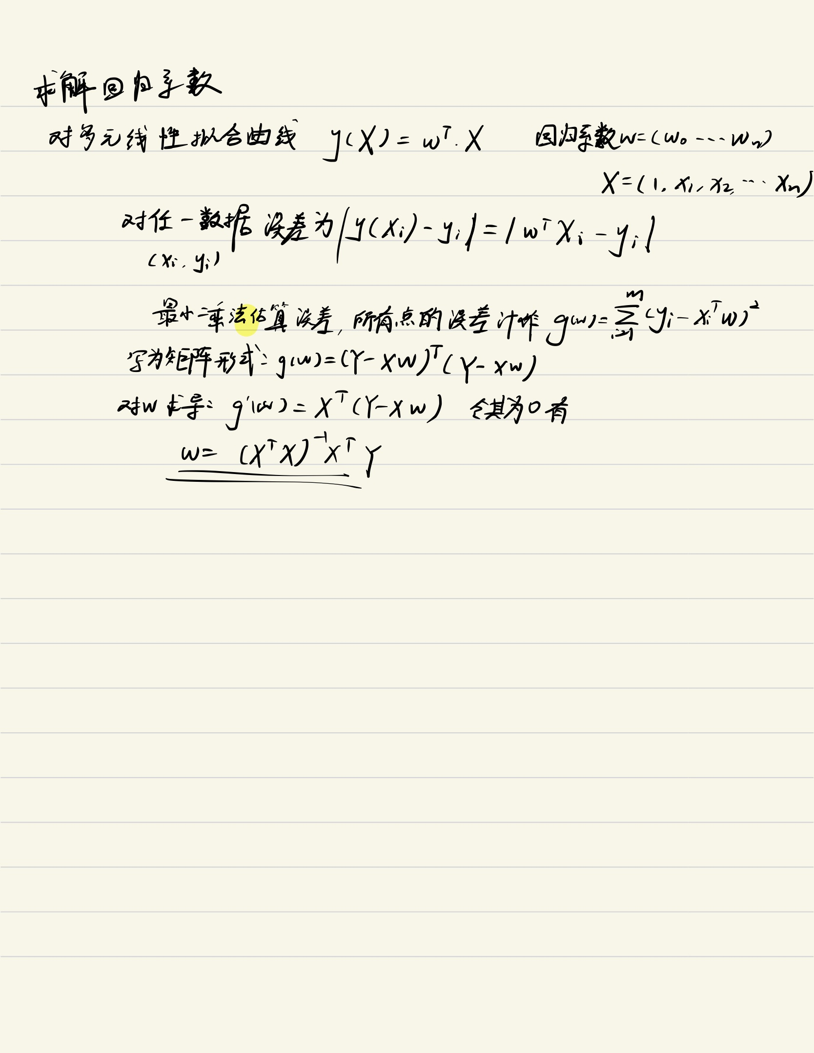

几个训练算法

最小均方算法（Least mean square，LMS算法）

大致思路：我们首先随便给θ一个初始化的值，然后改变θ值让J(θ)的取值变小，不断重复改变θ使J(θ)变小的过程直至J(θ)约等于最小值。
听着跟梯度下降差不多，其实就是损失函数为时的梯度下降，迭代公式为：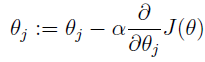
其中α为学习率。而其中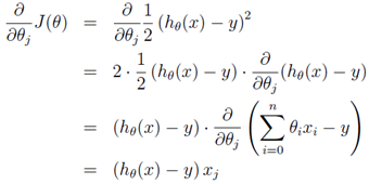
那么θ的迭代公式就变为：

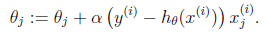
这是当训练集只有一个样本时的数学表达。当样本为多个时，涉及到梯度下降。

梯度下降

线性回归中的梯度下降不会像其他梯度下降那样陷入局部最优困境，因为其损失函数是二次凸函数，不会产生局部最优。但对多个样本的批梯度下降（batch gradient descent）计算量很大：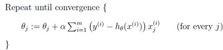
执行过程：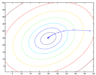

这时我们引入随机梯度下降（Stochastic Gradient Descent, SGD），我们在计算下降最快的方向时并不载入所有训练数据集，而是随机挑一个，这使计算量大大降低的同时较小地影响模型的准确性：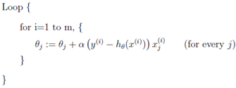


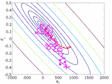
就像上图那样震荡趋向极小值点。

线性回归的Python实现

import numpy as np
from numpy.linalg import det
from numpy.linalg import inv
from numpy import mat
from numpy import random
import matplotlib.pyplot as plt
import pandas as pd

class LinearRegression:
    '''
    implements the linear regression algorithm class
    '''

    def __init__(self):
        pass

    def train(self, x_train, y_train):
        x_mat = mat(x_train).T
        y_mat = mat(y_train).T
        [m, n] = x_mat.shape
        x_mat = np.hstack((x_mat, mat(np.ones((m, 1)))))
        self.weight = mat(random.rand(n + 1, 1))
        if det(x_mat.T * x_mat) == 0:
            print 'the det of xTx is equal to zero.'
            return
        else:
            self.weight = inv(x_mat.T * x_mat) * x_mat.T * y_mat
        return self.weight

    def locally_weighted_linear_regression(self, test_point, x_train, y_train, k=1.0):
        x_mat = mat(x_train).T
        [m, n] = x_mat.shape
        x_mat = np.hstack((x_mat, mat(np.ones((m, 1)))))
        y_mat = mat(y_train).T
        test_point_mat = mat(test_point)
        test_point_mat = np.hstack((test_point_mat, mat([[1]])))
        self.weight = mat(np.zeros((n+1, 1)))
        weights = mat(np.eye((m)))
        test_data = np.tile(test_point_mat, [m,1])
        distances = (test_data - x_mat) * (test_data - x_mat).T / (n + 1)
        distances = np.exp(distances / (-2 * k ** 2))
        weights = np.diag(np.diag(distances))
        # weights = distances * weights
        xTx = x_mat.T * (weights * x_mat)
        if det(xTx) == 0.0:
            print 'the det of xTx is equal to zero.'
            return 
        self.weight = xTx.I * x_mat.T * weights * y_mat
        return test_point_mat * self.weight

    def lwlr_predict(self, x_test, x_train, y_train, k=1.0):
        m = len(x_test)
        y_predict = mat(np.zeros((m, 1)))
        for i in range(m):
            y_predict[i] = self.locally_weighted_linear_regression(x_test[i], x_train, y_train, k)
        return y_predict


    def lr_predict(self, x_test):
        m = len(x_test)
        x_mat = np.hstack((mat(x_test).T, np.ones((m, 1))))
        return x_mat * self.weight

    def plot_lr(self, x_train, y_train):
        x_min = x_train.min()
        x_max = x_train.max()
        y_min = self.weight[0] * x_min + self.weight[1]
        y_max = self.weight[0] * x_max + self.weight[1]
        plt.scatter(x_train, y_train)
        plt.plot([x_min, x_max], [y_min[0,0], y_max[0,0]], '-g')
        plt.show()

    def plot_lwlr(self, x_train, y_train, k=1.0):
        x_min = x_train.min()
        x_max = x_train.max()
        x = np.linspace(x_min, x_max, 1000)
        y = self.lwlr_predict(x, x_train, y_train, k)
        plt.scatter(x_train, y_train)
        plt.plot(x, y.getA()[:, 0], '-g')
        plt.show()

    def plot_weight_with_lambda(self, x_train, y_train, lambdas):
        weights = np.zeros((len(lambdas), ))
        for i  in range(len(lambdas)):
            self.ridge_regression(x_train, y_train, lam=lambdas[i])
            weights[i] = self.weight[0]
        plt.plot(np.log(lambdas), weights)
        plt.show()

def main():
    data = pd.read_csv('/home/LiuYao/Documents/MarchineLearning/regression.csv')
    data = data / 30
    x_train = data['x'].values
    y_train = data['y'].values
    regression = LinearRegression()
    # regression.train(x_train, y_train) 
    # y_predict = regression.predict(x_train)
    # regression.plot(x_train, y_train)
    # print '相关系数矩阵：', np.corrcoef(y_train, np.squeeze(y_predict))
    # y_predict = regression.lwlr_predict([[15],[20]], x_train, y_train, k=0.1)
    # print y_predict
    # regression.ridge_regression(x_train, y_train, lam=3)
    # regression.plot_lr(x_train, y_train)
    regression.plot_lr(x_train, y_train)

if __name__ == '__main__':
    main()